How to use this research compendium
comsldpsy.RmdThis research compendium comprises all the input and output files as well as the R code needed to reproduce our paper:
Visser, L., Kalmar, J., Linkersdörfer, J., Görgen, R., Rothe, J., Hasselhorn, M., & Schulte-Körne, G. (2020). Comorbidities between specific learning disorders and psychopathology in elementary school children in Germany. Frontiers in Psychiatry. http://doi.org/10.3389/fpsyt.2020.00292
The compendium uses the R package drake to define a reproducible processing pipeline linking inputs to outputs/targets similar to GNU make (for more information on the drake package, see here). This vignette describes how to reproduce the analysis, check the analysis pipeline, and inspect analysis steps and outputs.
Copy the analysis directory structure
After attaching the package, executing the function copy_analysis() copies the analysis directory structure to the current working directory (or an explicitely specified directory). The directory should now contain the following files:
.
└── .drake
    └── [...]
└── analysis
    ├── data
    │   └── data_orig.rds               # raw data
    ├── figures
    │   └── figure_1.tiff               # figures used in the manuscript
    │   └── figure_2.tiff
    │   └── figure_3.tiff
    ├── manuscript
    │   └── manuscript.docx             # manuscript as submitted
    │   └── supplemental.docx           # supplemental materials as submitted
    └── templates
        └── manuscript_template.docx    # manuscript template
        └── supplemental_template.docx  # supplemental materials template
These files represent all input files required to reproduce the analysis as well as all output files generated in the process. The function further copies a .drake directory to the same directory. This hidden directory stores information about the consistency of the analysis pipeline and all intermediate outputs.
Reproduce the analysis
Reproducing the analysis can be done in a two-step procedure:
-
Executing the function
reproduce_analysis()copies the analysis directory structure (if it isn’t already present) and then runsdrake::make(). The output provides evidence of reproducibility without actually re-running the analysis. If the analysis is reproducible, the output should look like this: -
To independently re-create the analysis results on ones own computer, one can run
reproduce_analysis()with the optionre_run = TRUE. This will delete the copied.drakefolder and re-run the entire analysis from scratch, re-creating all relevant intermediate steps and outputs.reproduce_analysis(re_run = TRUE) #> Reproducing analysis included in package 'comsldpsy': #> Analysis directory structure is already in place. #> Re-running analysis from scratch... #> target data_raw #> target manuscript_in #> target data_transformed #> target data_filtered #> [...] #> target manuscript_text #> target manuscript_tables #> target manuscript_figures #> target manuscript_out
Explore the analysis pipeline and results
Executing get_plan() returns the underlying drake plan used to run the analysis. The returned data frame lists all intermediate results (targets), the commands executed to create them, and the dependencies between them.
plan <- get_plan()
plan
#> # A tibble: 61 x 2
#>    target                                command
#>    <chr>                                 <chr>
#>  1 data_raw                              "readRDS(drake::file_in(\"analysis/da…
#>  2 data_transformed                      transform_data(data_raw)
#>  3 data_filtered                         filter_data(data_transformed, get_fil…
#>  4 df_correlation                        "get_corr_table(data_filtered, c(wllp…
#>  5 fisher_dsm5_cutoff_35_01_adhs_z_cat   "fisher_test(x = \"dsm5_cutoff_35_01\…
#>  6 fisher_dsm5_cutoff_35_01_des_z_cat    "fisher_test(x = \"dsm5_cutoff_35_01\…
#>  7 fisher_dsm5_cutoff_35_01_sca_e_z_cat  "fisher_test(x = \"dsm5_cutoff_35_01\…
#>  8 fisher_dsm5_cutoff_35_01_ssv_z_cat    "fisher_test(x = \"dsm5_cutoff_35_01\…
#>  9 fisher_dsm5_cutoff_35_math_adhs_z_cat "fisher_test(x = \"dsm5_cutoff_35_mat…
#> 10 fisher_dsm5_cutoff_35_math_des_z_cat  "fisher_test(x = \"dsm5_cutoff_35_mat…
#> # ... with 51 more rows
The drake package provides several ways to visualize the analysis pipeline, e.g.
Furthermore, drake provides functions for viewing individual targets (drake::readd()) or load them into the current environment (drake::loadd()).
For example, to view the cleaned data set, use:
readd(data_filtered)
#> # A tibble: 3,014 x 55
#>    gender grade       age land   analyze cft_iq_own_kl cft_impl cody_t_own
#>    <fct>  <fct>     <int> <fct>    <dbl>         <int> <fct>         <int>
#>  1 female 4. Klasse   122 Hessen       1           115 no               59
#>  2 male   3. Klasse   108 Bayern       1            99 no               41
#>  3 female 4. Klasse   121 Bayern       1           107 no               54
#>  4 female 4. Klasse   121 Hessen       1            77 no               46
#>  5 male   3. Klasse   106 Bayern       1            99 no               49
#>  6 female 3. Klasse   111 Bayern       1            96 no               44
#>  7 male   3. Klasse   111 Bayern       1            99 no               48
#>  8 female 4. Klasse   122 Bayern       1           107 no               58
#>  9 female 4. Klasse   126 Hessen       1            95 no               40
#> 10 male   4. Klasse   121 Bayern       1            86 no               44
#> # ... with 3,004 more rows, and 47 more variables: cody_z_own <dbl>,
#> #   cody_impl <fct>, wllp_t_own <int>, wllp_z_own <dbl>, wllp_impl <fct>,
#> #   childs_complete <int>, anamn_1 <fct>, anamn_24 <fct>, sca_e_z_own <dbl>,
#> #   des_z_own <dbl>, adhs_z_own <dbl>, ssv_z_own <dbl>, fbbssv_complete <int>,
#> #   anamn_12_c___15 <fct>, anamn_23_icd___44 <fct>, anamn_23_icd___70 <fct>,
#> #   anamn_23_icd___2 <fct>, anamn_23_icd___3 <fct>, anamn_23_icd___4 <fct>,
#> #   anamn_23_icd___5 <fct>, anamn_23_icd___54 <fct>, anamn_23_icd___55 <fct>,
#> #   anamn_23_icd___9 <fct>, anamn_23_icd___91 <fct>, anamn_23_icd___28 <fct>,
#> #   anamn_23_icd___48 <fct>, anamn_23_icd___80 <fct>, anamn_23_icd___83 <fct>,
#> #   anamn_23_icd___92 <fct>, anamn_23_icd___18 <fct>, wrt_t_own <dbl>,
#> #   wrt_z_own <dbl>, wrt_impl <chr>, nationality <fct>, education_mother <fct>,
#> #   dsm5_cutoff_35 <fct>, dsm5_cutoff_35_read <fct>,
#> #   dsm5_cutoff_35_spell <fct>, dsm5_cutoff_35_math <fct>,
#> #   dsm5_cutoff_35_01 <fct>, dsm5_cutoff_35_n <dbl>, dsm5_cutoff_35_012 <fct>,
#> #   sca_e_z_cat <fct>, adhs_z_cat <fct>, des_z_cat <fct>, ssv_z_cat <fct>,
#> #   psychopaths_n <dbl>
to view the results of the poisson regression model, use:
readd(df_poisson)
#> # A tibble: 2 x 5
#> term p.value estimate conf.low conf.high
#> <chr> <dbl> <dbl> <dbl> <dbl>
#> 1 (Intercept) 2.32e-138 0.454 0.427 0.483
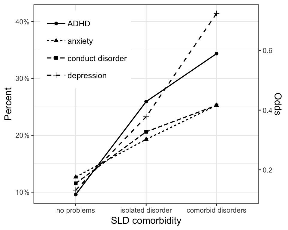
#> 2 dsm5_cutoff_35_n 2.20e- 43 1.66 1.55 1.79or, to view one of the figures included in the paper, use:
Cleaning up
Executing delete_analysis() removes the analysis and .drake directories from the working directory (or an explicitely specified directory).